Bayesian Partial Membership

Main Page

Generate samples for the Bayesian Partial Membership model using Hybrid Monte Carlo sampling.

Contents

Model Setup

Specify the data to use and the number of latent factors K. We generate 5000 samples. All HMC settings are specified in the configuration file.

dataName = 'bpmmodel';
model = 'bpm';
K = 3;
seed = 10;

[dataDir, outDir] = setupDir;
fileName = sprintf([outDir '/%s/%s_%s_%d_%d'], dataName,model, 'hmc', K, seed);

options = getConfigEFLVM(dataName, model);
burnin = options.burnin;
thin = options.thin;
saveOut = options.saveout;
setSeed(seed);

Load Data

data = getBinData(dataName, dataDir);
[N,D] = size(data.X);

Run EFA

Load a previously stored results if available

disp('Running HMC ...');
if ~exist([fileName,'.mat'],'file')
    %exptEFLVM(dataName,model,K, seed);
    inferFun = @inferBPM_hmc;
    predFun = @predProbBPM_mcmc;

    % Run HMC for few steps
    postDist = inferFun(data, options, K);

    % Save
    if saveOut, save(fileName, 'postDist', 'seed'); end

    % Test error
    if isfield(data,'miss')
        % only test if testing data exists
        [teErr, rmse, pHat] = predFun(data, postDist.samples, K, burnin, thin);
        if saveOut
            save(fileName,'teErr', 'rmse','-append');
        end;
    end;
end;

res = load(fileName);

Running HMC ...

Posterior Analysis

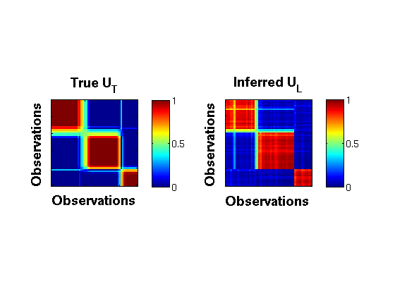
1. Comparing true vs inferred partial memberships

figure;
[S,LL] = size(res.postDist.samples);
gg = zeros(N,N);
burnin = 2000; thin = 50;
rng = burnin:thin:S;
for i = rng
    omega = res.postDist.samples(i,:);
    [~, ~, pi, ~] = extractParams_bpm(omega, K, N, D);
    gg = gg + pi*pi';
end;
GG = gg/length(rng);
TP = data.truePi*data.truePi';

r = 1; c = 2;
h1 = subplot(r,c,1);
imagesc(TP,[0 1]);
title('True U_T','FontSize',14, 'FontWeight','bold')
xlabel('Observations','FontSize',14, 'FontWeight','bold');
ylabel('Observations','FontSize',14, 'FontWeight','bold');
set(gca,'xticklabel',[],'yticklabel',[]);
ht = colorbar('location','EastOutside');
set(ht,'FontSize',12);
axis square;

h2 = subplot(r,c,2);
imagesc(GG,[0 1]);
title('Inferred U_L','FontSize',14, 'FontWeight','bold')
set(gca,'xticklabel',[],'yticklabel',[]);
% colormap gray;
xlabel('Observations','FontSize',14, 'FontWeight','bold');
ylabel('Observations','FontSize',14, 'FontWeight','bold');
ht = colorbar('location','EastOutside');
set(ht,'FontSize',12);
axis square;

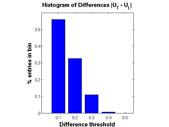
2. Histogram of Differences between above plots

figure;
diff = abs(GG(:) - TP(:));
rng = 0.1:0.1:0.5;
counts = histc(diff,rng);
perc = counts./sum(counts);
disp('Cumulative Histogram Table');
disp({'Perc. Values','Difference'});
disp([cumsum(perc)*100 rng']); % Print table instead

bar(rng,perc,'FaceColor','b');
title('Histogram of Differences |U_T - U_L|','FontSize',14, 'FontWeight','bold');
set(gca,'xtick',rng,'xticklabel',rng, 'FontSize',12)
xlim([0 0.55]); ylim([0 0.6]);
set(gca,'xtick',rng);
xlabel('Difference threshold','FontSize',14, 'FontWeight','bold');
ylabel('% entries in bin','FontSize',14, 'FontWeight','bold')
daspect([1 1 1])

Cumulative Histogram Table
    'Perc. Values'    'Difference'

           56          0.1
       88.571          0.2
       99.429          0.3
          100          0.4
          100          0.5

Shakir Mohamed, 2012

Published with MATLAB® 7.14